
Missing Value Handling Guide for ML Engineers

TL;DR:
- Handling missing data correctly involves diagnosing the underlying mechanism and choosing the appropriate imputation method accordingly. Imputing without understanding the cause of missingness leads to biased models and poor predictive performance. Using native support in models like XGBoost and LightGBM can eliminate the need for separate imputation steps.
Missing value handling is the process of identifying, diagnosing, and resolving gaps in a dataset before model training. Poor handling of null values is one of the most common causes of biased models and degraded prediction accuracy in production ML systems. The three core missing data mechanisms, MCAR (Missing Completely at Random), MAR (Missing at Random), and MNAR (Missing Not at Random), each demand a different response. This missing value handling guide covers how to diagnose which mechanism applies, select the right technique by missingness percentage, implement imputation without leaking data, and decide when native ML support makes separate imputation unnecessary.
What is the right missing value handling guide for your data?
The first step in any missing data strategy is diagnosing the mechanism. Skipping this step and jumping straight to mean imputation is the most common mistake ML engineers make.
- MCAR means missingness is unrelated to any observed or unobserved variable. A sensor randomly dropping readings is a classic example. Simple deletion or mean imputation is acceptable here.
- MAR means missingness depends on other observed variables. Income data missing more often for younger respondents is MAR if age is recorded. Model-based imputation using observed variables is the correct approach.
- MNAR means missingness depends on the missing value itself. High earners omitting salary data is MNAR. This requires specialized modeling or sensitivity analysis.
Diagnosing the mechanism requires more than intuition. Run correlation tests between missingness indicators and observed features. If a feature’s missingness correlates with another observed column, MAR is likely. If no pattern emerges across observed data, MCAR is plausible. MNAR is the hardest to confirm because the evidence is, by definition, absent.
Pro Tip: Create a binary missingness matrix and compute pairwise correlations with all observed features. Any correlation above 0.1 is a signal worth investigating before choosing your imputation method.

Misuse of imputation methods without understanding the underlying mechanism leads directly to biased models and invalid conclusions. Mechanism diagnosis is not optional preprocessing. It is the foundation of every decision that follows.
How does missingness percentage change your method choice?
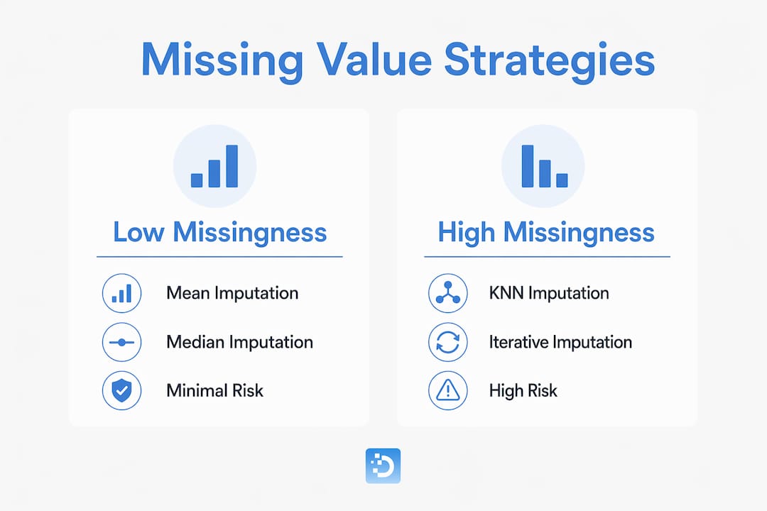
The proportion of missing values in a feature is the second axis of your decision. Mechanism tells you why data is missing. Percentage tells you how much you can recover.
| Missingness level | Recommended approach | Risk |
|---|---|---|
| Below 5% | Mean or median imputation | Minimal distributional distortion |
| 5%–20% | KNN or Iterative (MICE) imputation | Moderate complexity, manageable bias |
| Above 50% | Deletion or missing indicator feature | High risk of fabricating signal |
Simple imputation below 5% is widely accepted because the distributional impact is negligible. Mean imputation on a feature with 2% missing values will not meaningfully distort your model. The same approach on a feature with 30% missing values compresses variance and flattens correlations with the target.
For the 5%–20% range, KNN imputation uses the k nearest neighbors of each missing row to estimate the value. Iterative imputation, implemented as IterativeImputer in scikit-learn and based on MICE (Multiple Imputation by Chained Equations), cycles through features and fits a regression model for each. MICE handles complex missingness patterns more effectively than single-pass methods because it reconstructs the joint distribution across multiple iterations.
Above 50%, the math works against you. Imputing more than half a feature’s values means you are generating more signal than you observed. Deletion is acceptable only under MCAR with very low missingness. For high-missingness MNAR features, a binary missing indicator column often carries more predictive information than any imputed value.
How to implement imputation without introducing data leakage
Imputation errors in production almost always trace back to one mistake: fitting the imputer on the full dataset before splitting into train and test sets. This leaks test distribution information into training, inflating validation metrics and producing models that underperform in production.
- Split your data into train and test sets first, before any imputation.
- Fit your imputer (mean, KNN, or MICE) on the training set only.
- Apply the fitted imputer’s learned parameters to transform the test set.
- Wrap the entire sequence in a scikit-learn
Pipelineobject to enforce this order automatically.
Fitting imputers on training data only and applying learned parameters to test data is the correct pattern. A Pipeline makes this reproducible and eliminates the manual error risk.
The second common pitfall is treating imputation as a prediction task. Imputation is a distributional estimation task, not a prediction problem. Simple imputation reduces variability and distorts feature relationships. Optimizing an imputer for RMSE on held-out values produces point estimates that look accurate but compress the variance your model needs to learn from. Stochastic and multiple imputation approaches recover variability better than deterministic single-value methods.
For MNAR features, add a binary missing indicator column alongside the imputed values. Missing indicator features for MNAR data allow the model to learn from the pattern of absence itself, not just the imputed fill value. This is especially valuable in healthcare and finance datasets where the fact that a value is missing is often more informative than any plausible imputed substitute.
Pro Tip: When using MICE inside a scikit-learn Pipeline, set max_iter to at least 10 and check convergence by monitoring imputed value stability across iterations. Early stopping at the default setting often under-imputes complex missingness patterns.
Choosing the right method also requires considering dataset properties like size, variable distribution, and correlations. KNN imputation degrades on very large datasets because pairwise distance computation scales poorly. MICE is more stable at scale but computationally heavier. Match the method to your data’s actual properties, not just the missingness percentage rule of thumb.
Which ML algorithms handle missing values natively?
Several gradient boosting frameworks eliminate the need for a separate imputation step entirely. XGBoost, LightGBM, and CatBoost all natively handle missing values during tree construction by learning the optimal default direction for missing inputs at each split.
This native support differs from imputation in a fundamental way. Imputation fills gaps before training. Native handling lets the algorithm decide, during training, which branch a missing value should follow based on what minimizes loss. The model learns from missingness as a signal rather than treating it as a problem to be solved upstream.
Native missing data handling is the right choice when:
- Your dataset has moderate, scattered missingness across many features.
- You are using tree-based ensemble methods as your primary model class.
- You want to reduce preprocessing complexity in your AI-ready data pipeline.
The trend among ML engineers is shifting toward algorithms that manage missing data inherently, reducing reliance on external imputation pipelines. This does not mean imputation is obsolete. Linear models, neural networks, and distance-based algorithms still require complete feature matrices. For those model classes, imputation remains mandatory.
Comparing missing data handling strategies at a glance
| Method | Best for | Main risk |
|---|---|---|
| Listwise deletion | MCAR, very low missingness | Sample bias, reduced power |
| Mean/median imputation | Below 5% missingness, MCAR | Variance compression |
| KNN imputation | 5%–20%, MAR, moderate datasets | Slow on large data |
| MICE (iterative) | 5%–20%, MAR, complex patterns | Computationally intensive |
| Missing indicator | MNAR features, high missingness | Adds dimensionality |
| Native ML handling | Tree-based models, scattered gaps | Not available for all model types |
The right choice depends on your missingness mechanism, the percentage of missing values, and your model class. No single method wins across all scenarios. A solid data preprocessing workflow sequences these decisions deliberately rather than applying a single default.
Key Takeaways
Effective missing value handling requires diagnosing the missingness mechanism before selecting any technique, because the wrong method for the wrong mechanism produces biased models regardless of implementation quality.
| Point | Details |
|---|---|
| Diagnose before you impute | Identify MCAR, MAR, or MNAR before selecting any handling method. |
| Match method to missingness level | Use mean/median below 5%, KNN or MICE for 5%–20%, and indicators above 50%. |
| Prevent leakage in pipelines | Fit imputers on training data only and apply learned parameters to test sets. |
| Add missing indicators for MNAR | A binary absence flag often carries more signal than any imputed fill value. |
| Consider native ML support | XGBoost, LightGBM, and CatBoost handle missing inputs without separate imputation. |
What I’ve learned from watching imputation go wrong in production
The most expensive missing data mistakes I’ve seen don’t happen during model training. They happen six months later, when a feature’s missingness pattern shifts in production and the model silently degrades because nobody tracked it.
Imputation is not a one-time fix. It is a distributional assumption baked into your pipeline. When the real-world data generating process changes, your imputer’s learned parameters become stale. Mean values drift. Neighbor structures shift. MICE models trained on last year’s data impute values that no longer reflect current distributions.
The teams that handle this well treat imputation parameters as versioned artifacts, the same way they version model weights. They monitor missingness rates per feature in production and trigger retraining when rates deviate from training baselines. That discipline is rare, but it is the difference between a model that holds up and one that quietly fails.
My other strong opinion: resist the pull toward complexity. MICE is powerful, but mean imputation on a 2% missing feature is not a mistake. Spending engineering hours on a sophisticated imputation scheme for a low-missingness, MCAR column is waste. Reserve the heavy machinery for features where mechanism and percentage actually justify it.
— Oleg
How DOT Data Labs delivers datasets with missing data already resolved

Missing value handling is one of the most time-consuming steps in preparing training data, and it is also one of the most consequential. DOT Data Labs handles the full preprocessing chain for ML teams, including missingness diagnosis, imputation strategy selection, and quality validation before delivery. Every dataset DOT Data Labs produces goes through structured cleaning and deduplication, so your team receives model-ready training data without building or maintaining internal imputation pipelines. Whether you need an off-the-shelf dataset or a fully custom build, DOT Data Labs scopes each project against your model class, feature types, and missingness tolerance from day one.
FAQ
What is the difference between MCAR, MAR, and MNAR?
MCAR means missingness is random and unrelated to any variable. MAR means it depends on observed variables. MNAR means it depends on the missing value itself, making it the hardest to handle correctly.
When should I delete rows with missing values?
Deletion is safe only when data is MCAR and the missingness proportion is very low. Any other scenario risks sample bias and reduced statistical power.
What is MICE imputation?
MICE (Multiple Imputation by Chained Equations) is an iterative method that fits a regression model for each feature with missing values, cycling through features until imputed values stabilize. It handles complex missingness patterns better than single-pass methods.
Do I need to impute data when using XGBoost or LightGBM?
No. XGBoost, LightGBM, and CatBoost natively handle missing inputs by learning the optimal split direction for missing values during training. Separate imputation is not required for these model classes.
How do I prevent data leakage during imputation?
Fit your imputer on the training set only, then apply the learned parameters to the test set. Use a scikit-learn Pipeline to enforce this order and eliminate manual sequencing errors.